Data Preparation
The kind of data that we collected from the python script was very raw and needed a lot of work. For instance, the price was a character type and not an integer. Moreover, for any model to work efficiently, certain variables need to be introduced by combining or changing the existing variables.
This section focuses on various techniques we used to clean and prepare the data.
Generic Exploration & Cleaning
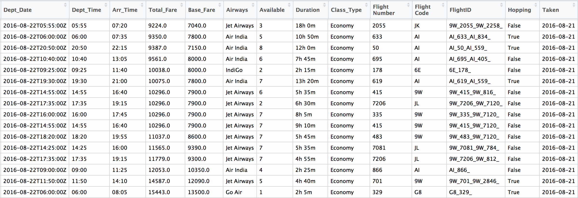
The collected data for each route looks like the one above. Because of the large number of flights in the busy routes like Delhi Bombay, the data collected over time is over a million points and hence efficiently handling such big data for faster computation is the first aim. In R the ‘fread’ function in ‘data.table’ package was used.
bomdel <- fread("bomdel.csv")A few basic cleaning and feature engineering looking at the data. A lot of data preparation needs to be done according to the model and strategy we use, but here are the basic cleaning we did initially to understand the data better:
-
Duplicates
There were not many, but a few repetitions in the data collected.
-
Days to departure
Our objective is to optimize this parameter. This the difference is the departure date and the day of booking the ticket. We consider this parameter to be within 45 days.
-
Day of departure
Intuitively we can say that flights scheduled during weekends will have a higher price compared to the flights on Wednesday or Thursday. Since including this in any of the models we use can be beneficial. We can also try to include the month or if it is a holiday time for better accuracy.
-
Duration
Converting the duration of the flight into numeric values, so that the model can interpret it properly. Also, it will be fair enough to omit flights with a very long duration.
-
Time of departure
Similar to day of departure, the time also seem to play an important factor. Hence we divided all the flights into three categories: Morning (6am to noon), Evening (noon to 9pm) and Night (9pm to 6am)
-
Hoppings
The data we collected did not give very authentic information about the number of hops a journey takes. Hence, we calculated the hops using the flight ids.
-
Outliers
We are focusing on minimizing the flight prices, hence we considered only the economy class with the following conditions:
a) The minimum value of total fare for all days for a particular flight id is less than the mean fare of all the flights b) The duration of the journey is less than 3 times the mean duration.
Data Specific Methods
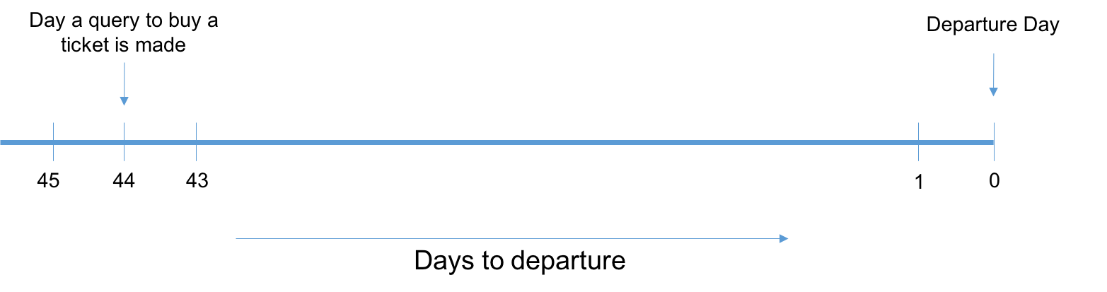
Suppose a user makes a query to buy a flight ticket 44 days in advance, then our system should be able to tell the user whether he should wait for the prices to decrease or he should buy the tickets immediately. For this we have two options:
- Predict the flight prices for all the days between 44 and 1 and check on which day the price is minimum.
- Classify the data we already have into, “Buy” or “Wait”. This then becomes a classification problem and we would need to predict only a binary number. However, this does not give a good insight on the number of days to wait.
For the above example, if we choose the first method we would need to make a total of 44 predictions (i.e. run a machine learning algorithm 44 times) for a single query. This also cascades the error per prediction decreasing the accuracy. Hence, the second method seems to be a better way to predict, wait or buy which is a simple binary classification problem. But, in this method, we would need to predict the days to wait using the historic trends.
For this we again have two options:
- We do the predictions for each flight id. The problem with this is that, if there is a change in flight id by the airline (which happens frequently) or there is an introduction or a new flight for a specific route then our analysis would fail.
- We group the flight ids according to the airline and the time of departure and do the analysis on each group. For this we need to combine the prices of the airlines lying in that group such that the basic trend in captured.
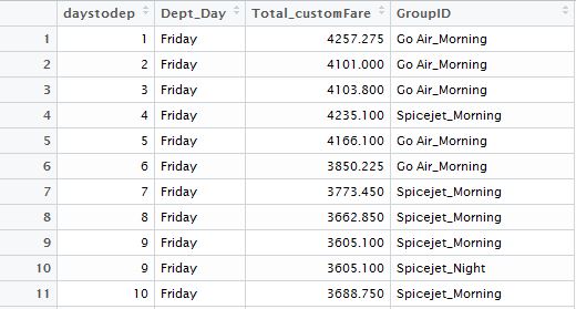
Moving ahead with the second option, we created the group according to the airlines and the departure time-slot created earlier (Morning, Evening, Night) and calculated the combined flight prices for each group, day of departure and depart day. Since these three are the most influencing factors which determine the flight prices. Also, we calculated the average number of flights that operated in a particular group, since competition could also play a role in determining the fare.
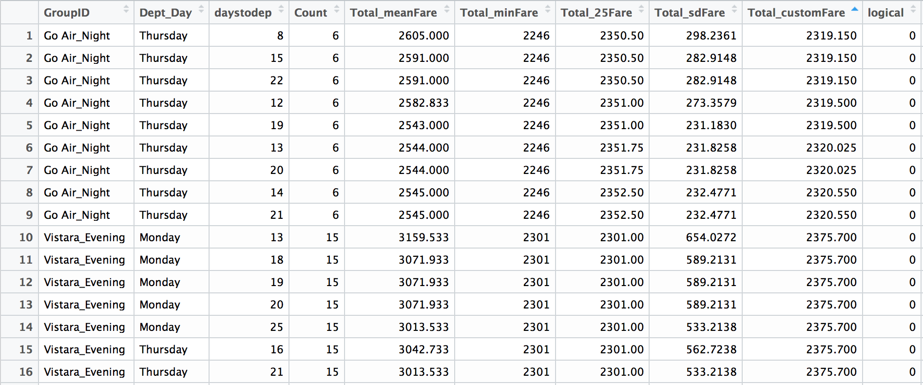
Combining fare for the flights in one group:
- Mean fare: This is the average of the fare of all the flights in a particular group corresponding to departure day and days to departure. Because of high standard deviation, taking the mean is not a very good option.
- Minimum fare: This does not give a very good insight of the trend, as a minimum value could occur because of some offer by an airline.
- First Quartile: This is a good measure as we are focusing on minimizing the fare and we do not want to consider the flights with high fares.
- Custom Fare: This is the fare giving more weightage to recent price trend.
Total_customFare = w*(First Quartile for entire time period) + (1-w)*(First quartile of last x days)
(We have considered: w = 0.7 and x = & days)
Calculating whether to buy or wait for the this data:
Logical = 1 if for any d < D the Total_customFare is less than the current Total_customFare
(Here, d is the days to departure and D is the days to departure for the current row.)
Trend Analysis
After creating the train file, we shift to create another dataset which is used to predict number of days to wait. For this, we used trend analysis on the original dataset.
Determining the minimum CustomFare for a particular pair of Departure Day and Days to Departure
We input the train dataset that has been created and find the minimum of the CustomFare corresponding to each combination of Departure Date and Days to Departure. Now with the obtained minimum CustomFare corresponding to each pair, we do a merge with our initial dataset and find out the Airline corresponding to which the minimum CustomFare is being obtained.
The count on the number of times a particular Airline appears corresponding to the minimum Custom Fare is the probability with which the Airline would be likely to offer a lower price in the future. This probability of each Airline for having a minimum Fare in the future is exported to the test dataset and merged with the same while the dataset of minimum Fares is retained for the preparation of bins to analyse the time to wait before the prices reduce
Creation of Bins
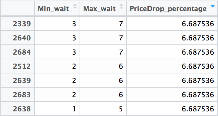
We next wanted to determine the trend of “lowest” airline prices over the data we were training upon. So the entire sequence of 45 days to departure was divided into bins of 5 days. In intervals of 5, the first bin would represent days 1-5, the second represents 6-10 and so on.
Corresponding to each bin, we required a value of the fare that would be optimal for consideration in suggesting a value for the days to wait to the user. Among all the points that lie in a bin, the 25th percentile was determined as the value that would be the possible lowest Fare corresponding to the bin which indicates days to departure.
Comparing the present price on the day the query was made with the prices of each of the bin, a suggestion is made corresponding to the maximum percentage of savings that can be done by waiting for that time period.The approximate time to wait for the prices to decrease and the corresponding savings that could be made is returned to the user.